Timothy Sauer

Numerical Analysis

Pearson New International Edition

• Broschiertes Buch

Produktbeschreibung

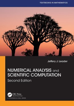
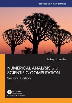
Numerical Analysis, Second Edition, is a modern and readable text for the undergraduate audience. This book covers not only the standard topics but also some more advanced numerical methods being used by computational scientists and engineers?topics such as compression, forward and backward error analysis, and iterative methods of solving equations?all while maintaining a level of discussion appropriate for undergraduates. Each chapter contains a Reality Check, which is an extended exploration of relevant application areas that can launch individual or team projects. MATLAB® is used throughout to demonstrate and implement numerical methods. The Second Edition features many noteworthy improvements based on feedback from users, such as new coverage of Cholesky factorization, GMRES methods, and nonlinear PDEs.

---

Hinweis: Dieser Artikel kann nur an eine deutsche Lieferadresse ausgeliefert werden.

Produktdetails

• Verlag: Pearson Education Limited
• 2 ed
• Seitenzahl: 612
• Erscheinungstermin: 2. August 2013
• Englisch
• Abmessung: 277mm x 223mm x 27mm
• Gewicht: 1280g
• ISBN-13: 9781292023588
• ISBN-10: 1292023589
• Artikelnr.: 48552716

Autorenporträt

Timothy Sauer earned his Ph.D. in mathematics at the University of California–Berkeley in 1982, and is currently a professor at George Mason University. He has published articles on a wide range of topics in applied mathematics, including dynamical systems, computational mathematics, and mathematical biology.

Inhaltsangabe

Preface
1. Solving Equations
2. Systems of Equations
3. Interpolation
4. Least Squares
5. Numerical Differentiation and Integration
6. Ordinary Differential Equations
7. Boundary Value Problems
8. Partial Differential Equations
9. Random Numbers and Applications
10. Trigonometric Interpolation and the FFT
11. Compression
12. Eigenvalues and Singular Values
References