
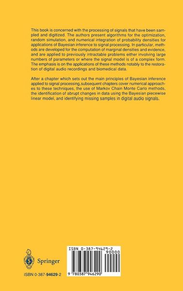
Numerical Bayesian Methods Applied to Signal Processing
-
- Hardcover ausgewählt
- Taschenbuch
- eBook
-
Sprache:Englisch
187,99 €
UVP
213,99 €
inkl. MwSt,
Lieferung nach Hause
Beschreibung
Details
Einband
Gebundene Ausgabe
Erscheinungsdatum
23.02.1996
Abbildungen
XIV, w. mit 118 Illustrationen 24,5 cm
Verlag
Springer UsSeitenzahl
244
Maße (L/B/H)
23,5/15,5/2 cm
Gewicht
565 g
Auflage
1996
Sprache
Englisch
ISBN
978-0-387-94629-0
Weitere Bände von Statistics and Computing
-
Numerical Analysis for Statisticians von Kenneth Lange
 - 13%
- 13%Kenneth Lange
Numerical Analysis for StatisticiansBuch
138,99 €
160,49 €* -
Automatic Nonuniform Random Variate Generation von Wolfgang Hörmann
 - 12%
- 12%Wolfgang Hörmann
Automatic Nonuniform Random Variate GenerationBuch
93,99 €
106,99 €* -
Software for Data Analysis von John Chambers
 - 13%
- 13%John Chambers
Software for Data AnalysisBuch
157,99 €
181,89 €* -
The Grammar of Graphics von Leland Wilkinson
 - 13%
- 13%Leland Wilkinson
The Grammar of GraphicsBuch
213,99 €
246,09 €* -
Modern Applied Statistics with S von W.N. Venables
 - 13%
- 13%W.N. Venables
Modern Applied Statistics with SBuch
157,99 €
181,89 €* -
S Programming von William Venables
 - 13%
- 13%William Venables
S ProgrammingBuch
101,99 €
117,69 €* -
Random Number Generation and Monte Carlo Methods von James E. Gentle
 - 13%
- 13%James E. Gentle
Random Number Generation and Monte Carlo MethodsBuch
119,99 €
139,09 €* -
The Basics of S-PLUS von Andreas Krause
 - 13%
- 13%Andreas Krause
The Basics of S-PLUSBuch
92,99 €
106,99 €* -
Numerical Linear Algebra for Applications in Statistics von James E. Gentle
James E. Gentle
Numerical Linear Algebra for Applications in StatisticsBuch
48,99 €
-
Introductory Statistics with R von Peter Dalgaard
Peter Dalgaard
Introductory Statistics with RBuch
58,99 €
-
Branch-and-Bound Applications in Combinatorial Data Analysis von Michael J. Brusco
 - 13%
- 13%Michael J. Brusco
Branch-and-Bound Applications in Combinatorial Data AnalysisBuch
101,99 €
117,69 €* -
Numerical Bayesian Methods Applied to Signal Processing von Joseph J.K. O. Ruanaidh
 - 12%
- 12%Joseph J.K. O. Ruanaidh
Numerical Bayesian Methods Applied to Signal ProcessingBuch
187,99 €
213,99 €*
Unsere Kundinnen und Kunden meinen
Verfassen Sie die erste Bewertung zu diesem Artikel
Helfen Sie anderen Kund*innen durch Ihre Meinung
Kurze Frage zu unserer Seite
Vielen Dank für dein Feedback
Wir nutzen dein Feedback, um unsere Produktseiten zu verbessern. Bitte habe Verständnis, dass wir dir keine Rückmeldung geben können. Falls du Kontakt mit uns aufnehmen möchtest, kannst du dich aber gerne an unseren Kund*innenservice wenden.
zum Kundenservice